

Noah’s Flood – Antediluvian Studies- Pre-Flood Conditions and Post-Flood Globe

Table of Contents
Overview – The Antedeluvian World
Historical sciences routinely reconstruct past environments using measurable present-day data, physical modeling, and experimental research. Geology, paleoclimatology, and evolutionary biology all infer ancient conditions by working backward from observable constraints. This article applies the same methodological approach to explore plausible environmental conditions before and immediately after the global Flood described in Genesis. The goal is not to claim direct observation of the pre-Flood world, but to examine what environmental states remain physically plausible under alternative chronological models. Measured data from geomagnetism, atmospheric physics, paleoclimate research, hyperbaric biology, solar variability studies, and tectonics provide constraints that can inform such reconstructions.

This study follows a structured progression: first examining geophysical and atmospheric variables that influence biological life; then evaluating transitional post-Flood conditions and large-scale geological reorganization; and finally reviewing historical interpretive models, including canopy hypotheses, within their proper evidential context. Throughout, a clear distinction is maintained between:
(1) directly measured scientific data,
(2) reasonable physical implications derived from that data, and
(3) speculative models proposed to explain biblical descriptions. The purpose is to explore how variations in boundary conditions could produce environmental states significantly different from those observed today. Reconstruction of ancient worlds—whether under conventional deep-time models or compressed chronologies—inevitably involves inference. The critical question is not whether inference occurs, but whether it remains grounded in measurable physical constraints. This article, therefore, approaches the subject with an evidence-first methodology, allowing implications to arise from established scientific principles rather than from unsupported assumptions.
(God) did not spare the ancient world, but preserved Noah, a herald of righteousness, with seven others, when he brought a flood upon the world of the ungodly – 2 Peter 2.5
The earth was formed out of water and through water by the word of God, and that by means of these the world that then existed was deluged with water and perished. – 2 Peter 3.5-6
Antediluvian Condition Reconstruction Model
Reconstructing environmental conditions prior to the Flood involves working backward from measurable physical constraints. This section examines geophysical, atmospheric, and biological variables that directly influence life on Earth. The objective is not to assert certainty regarding the pre-Flood world, but to explore which environmental states remain physically plausible when alternative chronological models are considered.
Geomagnetic Field and Radiation Environment
The Earth’s magnetic field plays a critical role in shielding the planet from charged solar particles and cosmic radiation. Modern measurements show that geomagnetic intensity varies over time and undergoes fluctuations in strength and polarity. Paleomagnetic studies indicate that field intensity has not been constant throughout Earth’s history, with periods of significantly stronger and weaker dipole strength documented in the geological record.
Measured modern trend: Direct observations indicate roughly a 10% decrease in dipole strength over the past ~180 years.

High-intensity evidence: Archaeomagnetic datasets from the Levant and Mesopotamia report multiple “geomagnetic spikes” between ~1050 and 600 BCE, with virtual axial dipole moment (VADM) reaching ~155–162 ZAm². The same study notes an increase from about 73 to 161 ZAm² between ~1750 and 1030 BCE, described as the largest Holocene intensity change in their curve.
Reference point: A commonly cited present-day dipole moment is about 7.8 × 10²² A·m² (≈ 80 ZAm²), which provides a useful baseline for comparison to paleointensity reconstructions.
Modern regression (first-order linear): If dipole strength fell ~10% over ~180 years, the implied linear slope is about −0.0556% per year (≈ −5.56% per century). This is a descriptive fit to the observed interval and is not assumed to apply indefinitely.
Chart: Geomagnetic Dipole Strength Across Geological Time
It is important to emphasize that the charts and datasets presented in this section are derived from mainstream geophysical and radiometric research. We are not introducing alternative measurements; we are evaluating existing data through a different chronological lens, i.e. Young Earth interpretation.
| Geologic Interval | Approx. Age (OE Model) | Dipole Moment (VADM, ZAm²) | Multiplier vs Modern (~80 ZAm²) | Notes |
|---|---|---|---|---|
| Modern Reference | Present | ~80 ZAm² | 1.0× | Current global dipole moment |
| Levant Geomagnetic Spike | ~1000 BCE | 155–162 ZAm² | ~1.9–2.0× | Significant uncertainty within the modern range |
| Late Proterozoic Interval | ~1.0 Ga | ~70–110 ZAm² | ~0.9–1.4× | Comparable to or modestly above modern |
| Mesoproterozoic Interval | ~1.5–2.0 Ga | ~60–100 ZAm² | ~0.75–1.25× | Variable, generally near modern magnitude |
| Paleoproterozoic | ~2.5 Ga | ~50–100 ZAm² | ~0.6–1.25× | Significant uncertainty within the modern range |
| Archean (zircon-based studies) | ~3.2–3.4 Ga | ~30–100 ZAm² | ~0.4–1.25× | Evidence for early active geodynamo |
Note: These spike values come from a high-resolution regional curve (Levant/Mesopotamia). The key claim is not that the entire globe must have matched the same peak everywhere, but that well-dated materials record intensity maxima substantially above modern values, providing an empirical upper bound for late Holocene field strength.
Archaeomagnetic reconstructions show that during several intervals between roughly 1050 and 600 BCE, the Earth’s dipole moment reached nearly twice modern strength. These values are not speculative—they are derived from laboratory measurements of baked clays, pottery, and other well-dated materials that preserve ancient magnetic signatures. Such data demonstrate that Earth’s magnetic field is capable of substantial intensity variation on century-scale timescales.
Implication A — shielding: A stronger geomagnetic dipole increases Earth’s shielding against charged particles, which in turn affects cosmic-ray penetration and cosmogenic isotope production. Holocene reconstructions and related work explicitly use geomagnetic field models to evaluate shielding effects and cosmogenic production variability, indicating the field strength is a meaningful control parameter in Earth’s near-space radiation environment. Laboratory and biomedical research demonstrate that ionizing radiation exposure contributes to DNA damage, mutation accumulation, and cellular stress.
Variations in geomagnetic shielding would therefore alter the radiation environment experienced by surface organisms. A stronger magnetic field would reduce cosmic ray penetration, while a weaker field would increase exposure. If geomagnetic intensity differed substantially prior to major geological reorganization events, this would plausibly affect long-term radiation exposure levels.
Implication B — direct biological interaction: Many organisms—including birds, marine animals, and certain bacteria—are known to detect and respond to Earth-strength magnetic fields for navigation (magnetoreception). Research on radical-pair mechanisms involving cryptochrome proteins demonstrates that biological systems are sensitive to magnetic fields in the microtesla range—the same magnitude as Earth’s field. This confirms that geomagnetic intensity operates within biologically active ranges.
Experimental research on static magnetic fields has also reported measurable effects on cellular growth, oxidative stress regulation, and certain healing processes under controlled conditions. While these findings do not establish that stronger geomagnetic intensity directly increases lifespan, they demonstrate that magnetic fields can influence biological processes at strengths comparable to Earth’s natural field.
Importantly, claims that a stronger magnetic field would directly produce extreme human longevity remain speculative. However, the magnetic field’s shielding effect is a measurable physical reality. Any reconstruction model involving a stronger dipole moment must account for its potential impact on radiation exposure and environmental stress levels.
Atmospheric Pressure and Hyperbaric Biology
Atmospheric pressure influences oxygen availability, gas exchange efficiency, and physiological stress responses in living organisms. Experimental hyperbaric research shows that elevated pressure environments can enhance oxygen diffusion in tissues and influence cellular repair processes under controlled conditions.
Chart: Published Geological Constraints on Ancient Atmospheric Pressure
Geological proxy studies do not support extreme multi-atmosphere ancient pressures. However, published upper bounds and modeling constraints indicate that moderate variations—up to approximately 1.5–2× modern pressure—remain within physically plausible limits in some interpretations of the geological record.
| Proxy Method | Approx Age (OE Model) | Inferred Pressure Range | Multiplier vs Modern (101 kPa) | Notes |
|---|---|---|---|---|
| Fossil Raindrop Imprints | ~2.7 Ga (Archean) | < 200 kPa (upper limit) | < 2.0× | Upper bound estimate; does not imply high sustained pressure |
| Basalt Vesicle Size Distribution | ~2.7 Ga | 50–200 kPa | 0.5×–2.0× | Based on gas bubble expansion modeling |
| Nitrogen Isotope Mass Balance | 1–3 Ga | Likely near modern | ~0.5×–1.5× | Suggests stable long-term N₂ inventory |
| Fluid Inclusions in Minerals | Various intervals | Generally near modern | ~1.0× | No evidence for extreme multi-atmosphere values |
Modern Reference: Mean sea-level atmospheric pressure today is approximately 101.3 kPa (1 atmosphere). Surface air density at sea level is approximately 1.225 kg/m³ at 15°C.
Plant growth studies conducted under varied atmospheric pressure and gas composition conditions demonstrate measurable changes in productivity, structural development, and water-use efficiency. These findings establish that atmospheric density and composition directly influence biological performance.
Chart: Medical Hyperbaric Effect
| Pressure Level | kPa | Multiplier vs Modern | Documented Effects |
|---|---|---|---|
| Modern Sea Level | 101 kPa | 1.0× | Baseline |
| Moderate Elevation (HBOT lower range) | 150 kPa | 1.5× | Improved oxygen diffusion, healing response |
| Medical Hyperbaric Treatment | 200–300 kPa | 2–3× | Enhanced tissue oxygenation, stress response modulation |
Environmental Implication: If atmospheric pressure in the past were moderately elevated (for example, 1.2–1.5× modern), this would increase air density, potentially enhancing aerodynamic lift, moisture retention, and gas diffusion efficiency. Such changes would influence ecosystem productivity and organism physiology.
Biological Implication: Controlled hyperbaric studies demonstrate that increased pressure enhances oxygen transport and can reduce hypoxic stress under specific conditions. While this does not prove extreme longevity, it establishes that atmospheric pressure is a biologically meaningful variable that affects tissue performance and stress response. Moderate variations within a factor of approximately 1–2× modern remain consistent with the evidence published concerning the model of the Earth’s past.
Oxygen Concentration and Oxidative Stress
Atmospheric oxygen concentration has varied throughout Earth’s geological past according to mainstream paleogeochemical models. Oxygen levels influence combustion thresholds, metabolic rates, and oxidative stress in biological systems. Experimental studies show that both hypoxic and hyperoxic conditions alter organism development and stress resilience. Atmospheric oxygen concentration directly influences metabolic efficiency, combustion thresholds, oxidative stress levels, and ecosystem productivity. Because oxygen plays a central role in cellular respiration and reactive oxygen species (ROS) generation, variations in atmospheric O₂ are biologically significant. Reconstruction of ancient oxygen levels relies on geochemical proxies rather than direct measurement.
Chart: Published Oxygen Level Estimates Through Time
It is important to emphasize that the charts and datasets presented in this section are derived from mainstream geophysical and radiometric research. We are not introducing alternative measurements; we are evaluating existing data through a different chronological lens, i.e. Young Earth interpretation.
| Geologic Interval (OE Model) | Approx. O₂ Estimate | Multiplier vs Modern (21%) | Proxy Basis |
|---|---|---|---|
| Modern | 21% | 1.0× | Direct measurement |
| Late Carboniferous (300 Mya) | 30–35% | 1.4–1.7× | Charcoal abundance, geochemical models |
| Mid-Cretaceous (150 – 60 Mya) | ~25% | ~1.2× | Biogeochemical modeling |
| Early Paleozoic (550 Mya) | 15–20% | 0.7–0.95× | Isotope modeling |
Physical Samples Used to Constrain Ancient Atmospheric Composition
| Sample Type | Approx Age (OE Model) | What Was Measured | Estimated O₂ | Notes / Limitations |
|---|---|---|---|---|
| Amber Gas Inclusions | Cretaceous–Cenozoic (140- 60 Mya) | Trapped microbubbles in fossil resin | ~18–23% | Diffusion possible; generally near modern values |
| Basalt Vesicle Imprints | Archean (~2.7 Ga) | Bubble size vs atmospheric pressure modeling | Indirect (pressure constraint) | Constrains total pressure, not directly O₂ % |
| Fluid Inclusions in Minerals | Various intervals | Entrapped gas/fluid chemistry | Near-modern composition | Possible alteration over time |
| Charcoal Abundance | Late Carboniferous (300 Mya) | Frequency of wildfire deposits | 30–35% | Indirect proxy; high O₂ increases flammability |
Modern Reference: Present atmospheric oxygen concentration is approximately 21% by volume (≈ 210,000 ppm).
The geological record demonstrates that atmospheric oxygen has fluctuated significantly, reaching up to approximately 1.5–1.7× modern levels during certain intervals. Such concentrations influence combustion dynamics, organism size, and metabolic performance. However, current evidence does not support extreme oxygen levels far beyond these ranges.
Chart: Experimental Effects of Elevated Oxygen
| O₂ Level | Multiplier vs Modern | Observed Biological Effects |
|---|---|---|
| 21% | 1.0× | Modern baseline |
| 25% | 1.2× | Increased metabolic capacity |
| 30–35% | 1.4–1.7× | Supports larger insect size; higher fire risk |
| >40% | >1.9× | Severe combustion instability; not ecologically stable |
Oxygen enables aerobic metabolism but also generates reactive oxygen species (ROS) as a byproduct. Elevated ROS contributes to cumulative cellular damage over time. Experimental research demonstrates that both low and excessively high oxygen levels can reduce organism lifespan, indicating an optimal biological range. Increased oxygen concentration enhances metabolic efficiency. Variations in oxygen levels would directly influence ecosystem productivity and organism physiology. Oxygen concentration remains a variable that must be constrained by both biological and geochemical considerations.
Greenhouse Gases and Climate Stability
Greenhouse gases regulate Earth’s surface temperature through radiative forcing. Carbon dioxide (CO₂), methane (CH₄), and water vapor (H₂O) absorb and re-radiate infrared energy, influencing global temperature gradients, precipitation patterns, and atmospheric circulation. Climate models demonstrate that modest variations in atmospheric composition can significantly influence global temperature gradients, precipitation patterns, and humidity levels.
Modern Reference:
- CO₂ : ~420 ppm
- CH₄ : ~1.9 ppm
- Water vapor: variable (0–4% by volume)
Chart: Published CO₂ Estimates Through Geological Time
| Geologic Interval (OE Model) | Estimated CO₂ (ppm) | Multiplier vs Modern (~420 ppm) | Proxy Basis |
|---|---|---|---|
| Modern | ~420 ppm | 1.0× | Direct measurement |
| Late Paleozoic (350 Mya) | 300–1,000 ppm | 0.7–2.4× | Stomatal density, carbon cycle models |
| Mesozoic (Warm Periods) (250 – 60 Mya) | 800–2,000 ppm | 2–5× | Marine carbonates, geochemical modeling |
| Early Paleozoic (550 Mya) | 1,000–3,000 ppm | 2–7× | GEO-CARB-SULF modeling |
Radiative forcing relationship (simplified): [ ΔF ≈ 5.35ln (C/Co) ]Where:
- C = CO₂ concentration
- C0 = baseline concentration
- ΔF = radiative forcing (W/m²)
This shows:
- CO₂ forcing increases logarithmically.
- Doubling CO₂ does not double the temperature.
- The effect saturates gradually.
Experimental and Observational Effects
Greenhouse variation influences:
- Global temperature gradients
- Polar ice stability
- Rainfall distribution
- Plant growth (CO₂ fertilization effect)
Experimental plant studies consistently show:
- Elevated CO₂ increases photosynthetic efficiency.
- Water-use efficiency improves.
- Growth rate often increases under moderate elevation (2×–3× modern).
Chart: Documented Biological Effects of Elevated CO₂
It is important to emphasize that the charts and datasets presented in this section are derived from mainstream geophysical and radiometric research. We are not introducing alternative measurements; we are evaluating existing data through a different chronological lens, i.e. Young Earth interpretation.
| CO₂ Level | Multiplier vs Modern | Observed Effects |
|---|---|---|
| 420 ppm | 1.0× | Modern baseline |
| 800 ppm | ~2× | Increased photosynthesis, improved water efficiency |
| 1,200–1,500 ppm | 3–4× | Enhanced plant growth in controlled experiments |
| >3,000 ppm | >7× | Potential thermal instability depending on feedbacks |
Geological reconstructions indicate that CO₂ levels have varied significantly throughout Earth’s history, often exceeding modern concentrations by factors of 2–5× during certain intervals. Such concentrations would produce warmer global climates and enhanced hydrological cycling under established radiative principles. Moderate greenhouse enhancement can increase plant productivity and ecosystem density. However, extreme greenhouse concentrations would introduce thermal instability and are constrained by climate feedback mechanisms. Reconstruction models must remain within physically stable bounds.
Landmass Configuration and Ocean Circulation

The distribution of continents influences ocean currents, atmospheric circulation, rainfall patterns, and global temperature gradients. Even within conventional tectonic models, changes in continental arrangement are known to significantly alter climate behavior. Therefore, any reconstruction of ancient environmental conditions must consider how landmass configuration affects oceanic heat transport and ecological stability. The distribution of continents influences ocean currents, atmospheric circulation, rainfall belts, and climate stability. Even within conventional tectonic models, continental arrangement dramatically alters heat transport and biome distribution.
Chart: Climate Effects of Major Continental Arrangements
Ocean currents redistribute solar heat from equatorial regions toward the poles. Modern example:
- Gulf Stream transports ~1 petawatt of heat northward.
- Thermohaline circulation regulates deep ocean temperatures.
Small changes in basin geometry can strengthen or weaken heat transport, alter polar ice stability, and modify precipitation patterns. Climate models show that:
- Rearranging continents can shift the global mean temperature by several degrees Celsius.
- Ocean gateway changes can dramatically alter regional climates.
- Polar amplification depends heavily on ocean circulation strength.
| Configuration | Documented Climate Effect | Mechanism |
|---|---|---|
| Supercontinent (Pangaea) | Strong interior aridity | Reduced coastal moisture transport |
| Panama Seaway Closure | Altered Atlantic circulation | Changed thermohaline flow patterns |
| Antarctic Isolation | Glaciation onset | Circumpolar current formation |
| Fragmented Continents | More maritime climate influence | Increased coastal moderation |
Landmass configuration influences:
- Habitat continuity
- Species migration corridors
- Climate uniformity
- Rainfall distribution

A more contiguous landmass could reduce extreme seasonal gradients in certain regions and alter biome distribution. A fragmented system increases coastal moderation and regional climate diversity. A different landmass configuration prior to major tectonic reorganization events would plausibly affect regional climate uniformity, habitat connectivity, and species dispersion patterns. Climate simulations consistently demonstrate the sensitivity of global weather systems to continental geometry.
Rearrangement of ocean basins and landmasses alters heat transport efficiency, atmospheric circulation, and ecological stability. Therefore, reconstruction of ancient environmental conditions must account for potential differences in continental geometry and ocean circulation. Because ocean heat transport strongly influences polar stability and rainfall distribution, changes in basin geometry can produce significantly different climate regimes even under similar greenhouse gas concentrations. Such variability provides a physically grounded mechanism for environmental differences between geological intervals.
Earth’s Early Ocean
The Jack Hills zircon evidence places important constraints on early Earth models. Elevated δ¹⁸O values indicate that liquid water and surface weathering processes were already active by approximately 4.3–4.4 billion years ago. This challenges earlier models that proposed a prolonged, globally molten surface and delayed crust formation. While it does not eliminate the possibility of an initial magma ocean phase, it significantly shortens the timeframe during which extreme surface temperatures could have persisted.

Zircon Oxygen Isotope Evidence for Early Surface Water
| Sample Type | Approx Age (Ga) (OE Model) | δ¹⁸O Signature | Interpretation |
|---|---|---|---|
| Jack Hills Zircon | 4.3–4.4 Ga | Elevated above the mantle baseline | Interaction with liquid water |
| Mantle-derived Zircon (reference) | Various | ~5.3‰ | No surface water alteration |
This evidence supports:
- Early liquid water
- Early crust stability
- Early hydrological cycling
Evidence for Pre-Flood Landmass Configuration and Marine Redistribution
Carboniferous coal-bearing strata are widely distributed across present-day continents, including North America, Europe, and Asia. These deposits represent large accumulations of plant biomass that were buried and preserved. In addition, many coal-bearing formations extend beneath modern continental shelves, indicating that depositional environments have shifted significantly relative to present coastlines.
The broad geographic distribution of plant-derived carbon deposits, particularly coal-bearing strata, indicates that extensive vegetated ecosystems once occupied regions that are now widely separated by oceans. In conventional geological interpretation, this pattern is explained through continental drift and paleogeographic reconstructions such as the supercontinent Pangaea, in which presently distant landmasses were once joined and supported continuous biomes.
Within a Young Earth reconstruction framework, the same distributional data may be understood differently. Rather than requiring hundreds of millions of years of tectonic separation, these widespread carbon deposits may reflect a pre-Flood world characterized by more continuous continental surfaces and expansive vegetated regions that were subsequently fragmented and reorganized during large-scale hydrological and tectonic events. At minimum, the scale of preserved plant carbon suggests either broader contiguous land areas or ecosystems capable of sustaining exceptionally dense and productive foliage across extensive regions.
The Ocean May Have Been Less Salty
Given that ocean salinity depends on erosion rates, basin geometry, and tectonic recycling efficiency, it is reasonable to examine whether earlier marine conditions could have been significantly less saline than modern oceans; a full treatment of this idea is developed in a companion article:
Soil Fertility, Productivity, and Extrapolation from Modern Analogs
Modern ecology demonstrates that exceptionally productive ecosystems do not require unusually nutrient-rich parent material. In many regions, high biomass is sustained by efficient nutrient cycling rather than by high baseline nutrient concentrations in the soil itself. Tropical forest systems can maintain dense vegetation even where soils are highly weathered and relatively nutrient-poor, because nutrients are rapidly recycled through organic matter, microbial communities, and root–fungal networks. In addition, multiple well-studied examples show that soil fertility can be significantly increased and stabilized when carbon-rich organic inputs and mineral amendments are added over time.
Chart: Documented Ancient Nutrient-Enriched Soils (Measured Data)
| Region | Soil Type / Context | Approx. Age | Measured Nutrient Difference vs. Surrounding Soils | Notes |
|---|---|---|---|---|
| Amazon Basin | Terra Preta | ~7,000–2,500 years BP | • 2–3× higher organic carbon • Up to 3–6× higher phosphorus • Elevated Ca, K • Up to 70× higher black carbon | Anthropogenic biochar + organic waste; persistent fertility for centuries |
| Colca Valley | Ancient agricultural terraces | ~1,500 years BP | • Higher total nitrogen • Elevated available phosphorus • Increased organic carbon | Long-term soil retention & organic amendments |
| Chesapeake Bay | Prehistoric shell middens | ~1,000–3,000 years BP | • 4–16× higher phosphorus • Elevated calcium • Higher pH (less acidic) | Shell, bone, ash accumulation; long-lasting fertility enhancement |
| Tanzania | Pastoral Neolithic midden soils | ~3,000–5,000 years BP | • 2–5× higher phosphorus • Elevated nitrogen • Increased organic matter | Livestock waste accumulation & long-term settlement sites |
| Hawaii | Traditional agroforestry systems | ~500–1,500 years BP | • Increased phosphorus • Improved cation exchange capacity • Higher organic carbon in managed systems | Volcanic mineral crushing + organic inputs |
Amazonian Terra Preta (“dark earth”) soils exhibit markedly higher organic carbon and increased concentrations of plant-available nutrients such as phosphorus, calcium, and potassium compared to adjacent soils, and this enhanced fertility can persist for centuries to millennia. Similar long-lasting nutrient enrichment has been documented in ancient agricultural terraces (where soil retention and organic inputs improve fertility) and in prehistoric midden sites (where shell, bone, ash, and organic waste elevate calcium, phosphorus, and pH buffering). These cases establish two important constraints:
- (1) high productivity can be maintained without globally “rich” soils when nutrient cycling is efficient, and
- (2) nutrient retention and fertility can be increased and preserved for long periods under stable ecological conditions with sustained organic input.
Given the evidence that (a) soil fertility can be stabilized for long durations under favorable conditions, and (b) past ecosystems produced biomass at continental scales, it is reasonable within a reconstruction framework to explore how pre-Flood boundary conditions might have supported higher average productivity than many modern landscapes.
Radiation – Solar and Space Weather Influences
Solar radiation and charged particle flux are primary external drivers of Earth’s atmospheric and surface environment. Variations in solar output influence climate forcing, atmospheric ionization, and cosmic ray penetration. Because the geomagnetic field interacts directly with solar wind and heliospheric conditions, reconstruction of ancient environmental states must also consider solar variability and space weather dynamics. Solar variability influences atmospheric ionization and radiation flux at Earth’s surface. Changes in magnetic shielding, solar output, or heliospheric modulation affect cosmic ray penetration. Cosmogenic isotope records demonstrate that solar activity fluctuates over time.

Modern Solar Cycle: Direct satellite measurements show that total solar irradiance varies by approximately 0.1% over the 11-year solar cycle. Although small in energy percentage, associated changes in solar magnetic activity significantly alter charged particle flux and space weather conditions.
Chart: Solar Activity Proxies
| Proxy | What It Indicates | Timescale (Oe Model) |
|---|---|---|
| Sunspot Records | Magnetic activity level | ~400 years (instrumental) |
| Carbon-14 in Tree Rings | Cosmic ray flux variation | ~10,000 years |
| Beryllium-10 in Ice Cores | Solar modulation strength | ~100,000+ years |
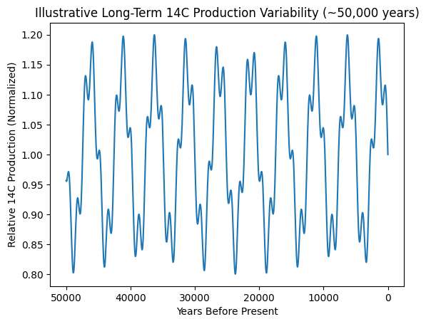
C14 DataSet Timeline (IntCal)
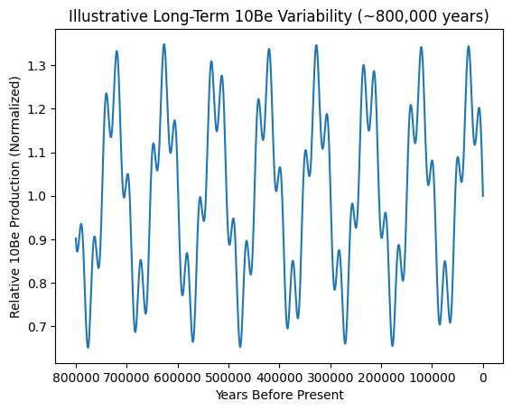
BE10 DataSet Timeline (IntCal)
Stellar evolution models indicate that the early Sun’s total luminosity was approximately 20–30% lower than present levels during the early years of Earth’s history. This so-called “Faint Young Sun” condition demonstrates that solar output is not static over time. While luminosity and high-energy particle radiation are governed by different mechanisms, the broader point remains that solar forcing parameters have varied throughout Earth’s past, contributing to changing boundary conditions that influence atmospheric chemistry, shielding efficiency, and surface radiation environments.
Standard stellar models indicate that solar luminosity has increased over time, with the early Sun emitting significantly less total radiant energy than today. Although luminosity does not directly equate to cosmic radiation intensity, this confirms that solar forcing is not constant and that environmental radiation conditions must be evaluated as time-dependent variables rather than fixed constants.
Cosmic Ray Proxies: Cosmogenic isotopes such as carbon-14 (¹⁴C) in tree rings and beryllium-10 (¹⁰Be) in ice cores provide measurable records of cosmic ray flux. Variations in these isotopes reflect changes in solar magnetic activity and geomagnetic shielding strength. Periods of stronger geomagnetic intensity and enhanced solar magnetic activity reduce cosmic ray penetration into the lower atmosphere. Because ionizing radiation contributes to DNA damage and oxidative stress, changes in magnetic shielding have measurable biological relevance.
Ionizing radiation is known to cause DNA strand breaks and increase mutation rates. Organisms possess repair mechanisms that mitigate daily radiation damage. Variations in geomagnetic strength and solar magnetic activity would influence background radiation exposure and could alter cumulative biological stress over long intervals. However, current evidence does not allow precise quantification of ancient surface radiation levels beyond proxy inference.
Biological Resilience and Environmental Stressors

Biological systems operate within defined environmental thresholds. Temperature, radiation exposure, atmospheric composition, pressure, and nutrient availability all influence cellular stability, metabolic efficiency, mutation rates, and organism longevity. Reconstruction of ancient environmental conditions, therefore, requires consideration of how these physical parameters interact with biological resilience mechanisms. Modern lifespan and organism resilience are influenced by cumulative environmental stressors, including radiation exposure, pathogen load, oxidative stress, and nutritional stability. Variations in climate stability, radiation shielding, and atmospheric composition would plausibly influence these factors.
Ionizing radiation induces DNA strand breaks and oxidative damage. Organisms possess repair systems, including base excision repair, nucleotide excision repair, and double-strand break repair pathways. Background radiation levels influence cumulative mutation load over time, although biological repair mechanisms mitigate most routine damage.
Atmospheric pressure affects gas solubility, diffusion gradients, and respiratory efficiency. Experimental studies demonstrate that moderate variations in pressure alter oxygen delivery and metabolic performance. However, extreme pressure deviations introduce physiological instability.
Elevated CO₂ concentrations are experimentally shown to enhance photosynthetic efficiency and water-use effectiveness in many plant species. Increased primary productivity alters ecosystem density and trophic structure. However, these effects are nonlinear and constrained by nutrient availability and climatic stability.
Environmental stressors do not act independently. Radiation exposure, atmospheric composition, temperature gradients, and geomagnetic shielding interact dynamically. Variations in these parameters influence mutation rates, metabolic burden, and ecological productivity. While existing data do not permit precise quantification of ancient biological stress levels, it is clear that environmental variables affecting cellular resilience are not static over time. While extreme lifespan claims remain outside direct experimental verification, it is well established that environmental conditions influence genetic stability and population health. Reconstruction models, therefore, examine whether combinations of altered boundary conditions could produce measurably different biological baselines.
Alignment to Biblical Context
Within a Biblical framework, such environmental variability is sometimes considered in discussions of the gradual reduction in recorded human lifespans following the early genealogical accounts (e.g., Genesis 47:9), not as a direct scientific proof of extended longevity, but as a potential contextual factor consistent with the observed pattern of declining years.
While environmental factors alone cannot be shown to account for the extended lifespans recorded in early Genesis, the documented variability of radiation exposure, atmospheric composition, and geomagnetic shielding provides a reasonable physical context in which differing biological baselines may have existed. This perspective aligns with the Biblical record’s depiction of declining lifespans across generations (Genesis 47:9), without requiring claims beyond what the data can directly demonstrate.
“The days of the years of my pilgrimage are one hundred and thirty years; few and evil have been the days of the years of my life, and they have not attained to the days of the years of the life of my fathers in the days of their pilgrimage.” – Joseph speaking to Pharaoh, Genesis 47.9
Post-Flood Transition Conditions and Deluvian Reorganization

Modern Earth science documents multiple classes of high-energy sedimentary processes capable of large-scale erosion and rapid burial. Megaflood systems such as those associated with the Channeled Scablands of Washington demonstrate that catastrophic water discharge can excavate deep channels, transport enormous sediment volumes, and reshape regional topography in relatively short timeframes. Peak discharge estimates for Missoula-type floods exceed 10 million cubic meters per second, orders of magnitude greater than any modern river system.
Within conventional geological frameworks, these high-energy processes are typically interpreted as regional events distributed over extended geologic timescales. Megafloods, turbidity currents, delta collapses, and basin infill episodes are viewed as episodic disturbances embedded within longer-term depositional regimes. However, the physical mechanisms themselves do not require slow accumulation. The evidence demonstrates that:
- Large volumes of sediment can be mobilized quickly.
- Thick stratified sequences can form under high-energy conditions.
- Fine lamination does not inherently require annual or seasonal deposition.
- Deep erosional features can develop during extreme discharge.
The interpretive divergence arises primarily in the temporal organization of these processes. In a Young Earth Biblical framework, the Genesis Flood narrative describes sustained global-scale hydrological disruption involving intense rainfall and subterranean water release. If such an event occurred, it would produce conditions capable of generating repeated high-energy sediment transport across continental margins and ocean basins. Under this view, many large sedimentary packages are interpreted not as isolated regional events separated by millions of years, but as components of a coherent global hydrodynamic episode followed by decaying instability.
The geological record already demonstrates that catastrophic erosion and rapid sedimentation occur. The Young Earth interpretation proposes that such processes were not merely regional anomalies, but globally synchronized within a short interval. This establishes the physical foundation for the broader post-Flood reorganization phase, including tectonic uplift, climate volatility, and ecological reset.
Length of Noah’s Flood
How Long Did Noah’s Flood Last? If we do the calculation in the Bible, we can determine just how long exactly Noah’s flood took place for. [Genesis 7 &8]:
- Noah was 600 years old when the flood waters began
- In his 600th year, 2nd month, and 7th day, the fountains of the deep broke open, and the windows of heaven were opened.
- It rained for 40 days and nights.
- After it rained, the waters prevailed for another 150 days (5 months)
- The water covered the highest mountain tops by a depth of 45 feet.
- At the end of the 150 days, the Ark grounded on the 17th day of the 7th month.
- Waters receded for 2 months until the 1st day of the 10th month, in which the tops of the mountains were exposed.
- 40 days after the mountains were seen, Noah sent out a dove, but it returned not able to find land.
- A week later, he sent a dove out again, which returned with an olive branch.
- Another week followed, and he sent it out again, and it did not return.
- In the 601st year, 1st month, 1st day on Noah’s birthday, he saw that the face of the ground was dry, but not yet firm.
- He waited 1 more month on the 27th day, and God commanded Noah to leave the Ark.
- Total time from Noah entering the Ark 2026 to the time of departure 2026:
- = 1 year, 0 months, 10 days.
Mountain Uplift and Orogenic Pulses
Mountain building (orogeny) is not observed as a smooth, constant-rate process. Geological and geophysical research consistently demonstrates that uplift occurs in pulses associated with tectonic reorganization, crustal thickening, slab dynamics, and isostatic adjustment. Several independent methods document episodic uplift:
- Thermochronology (apatite fission-track, (U-Th)/He dating)
- Sediment provenance analysis
- Structural deformation studies
- Stratigraphic relationships and angular unconformities
- GPS measurements (modern vertical displacement)
Modern GPS networks measure vertical crustal movements in tectonically active regions ranging from millimeters to centimeters per year. Over short geological intervals, such rates can translate into substantial elevation change. Thermochronologic studies in major mountain belts (e.g., Himalayas, Andes, Alps) indicate accelerated exhumation phases, sometimes interpreted within conventional timescales as rapid uplift events relative to background rates. Mountain belts do not rise at perfectly uniform rates.
Major Mountain Systems — Initial Orogeny vs. Final Elevation Phase
Conventional Old Earth Geological Timescale
| Region | Mountain Chain / Plateau / Rift | Initial Major Orogenic Phase (OE Model) | Major Late Elevation / Relief Phase (OE Model) | Notes |
|---|---|---|---|---|
| Europe | Swiss Alps | ~65–30 Ma | < 2–5 Ma | Significant late exhumation and relief development |
| Apennines | ~23 Ma | 1–5 Ma | Neogene uplift phase | |
| Pyrenees | ~65–25 Ma | 2–5 Ma | Late uplift following collision | |
| Baetic Cordillera | ~30–20 Ma | 2–5 Ma | Neogene tectonic reactivation | |
| Carpathians | ~30–10 Ma | 2–5 Ma | Late Neogene uplift | |
| Caucasus | ~25–15 Ma | < 2–3 Ma | Ongoing uplift | |
| Ural Mountains | ~300–250 Ma | Minor later reactivation | Ancient core, heavily eroded | |
| Sudeten Mountains | Paleozoic (~300 Ma) | 1–5 Ma | Reactivated uplift | |
| Asia | Tibetan Plateau | ~50–40 Ma | < 3–5 Ma | Major plateau elevation increase in Neogene |
| Himalayas | ~50 Ma | < 3–5 Ma | Accelerated uplift; ongoing | |
| Kunlun Mountains | ~40–30 Ma | < 4 Ma | Reactivated uplift phase | |
| Tien Shan | Paleozoic (~300 Ma) | < 2–3 Ma | Strong Neogene reactivation | |
| Shanxi Mountains | ~30 Ma | < 3 Ma | Cenozoic uplift | |
| Japanese Mountains | ~20–15 Ma | < 5 Ma | Active island arc uplift | |
| Taiwan Mountains | < 10 Ma | < 5 Ma | Very young high-relief orogen | |
| North America | Sierra Nevada | ~100 Ma (batholith formation) | < 2–5 Ma | Significant late uplift and tilting |
| Colorado Plateau | ~70–40 Ma | < 3–6 Ma | Major incision linked to uplift | |
| Bighorn Mountains | ~70 Ma | < 3–5 Ma | Reactivated uplift | |
| Rocky Mountains | ~80–40 Ma | < 5–10 Ma | Modern elevation partly late | |
| Canadian Cordillera | ~60 Ma | 2–5 Ma | Late uplift and exhumation | |
| Cascade Range | < 20 Ma | 4–5 Ma | Volcanic arc elevation phase | |
| South America | Chilean Andes | ~60 Ma | < 5–10 Ma | Late Cenozoic uplift pulse |
| Bolivian Andes | ~40 Ma | < 5–10 Ma | Plateau elevation increase | |
| Ecuadorian Andes | ~40 Ma | < 5–10 Ma | Active arc uplift | |
| Africa | Ethiopian Rift | ~30 Ma | < 3–5 Ma | Rift-related uplift |
| Western Rift (East Africa) | ~30 Ma | < 3–5 Ma | Ongoing uplift | |
| Ruwenzori Mountains | Rift onset ~30 Ma | < 3 Ma | Rapid block uplift | |
| Other | New Guinea Mountains | < 10 Ma | ~2–5 Ma | Rapid modern uplift |
| New Zealand Southern Alps | < 25 Ma | < 5 Ma | Rapid uplift; high modern rates |
Although conventional models distribute these uplift phases across millions of years, the concentration of major elevation-building events within the Late Cenozoic interval is striking. The fact that many of the world’s highest relief mountain systems achieved substantial elevation during the same broad geological window suggests a globally coordinated tectonic reorganization rather than purely isolated local events. Within a Young Earth framework, this clustering is interpreted as evidence of rapid post-Flood lithospheric stabilization rather than prolonged incremental uplift. Under a compressed post-Flood framework:
- Lithospheric instability following global crustal disruption
- Rapid plate reorganization
- Isostatic rebound from massive sediment redistribution
- Thermal disequilibrium in oceanic crust

Marine fossils preserved within limestone near the summit of Mount Everest demonstrate that rocks now standing at the highest elevations on Earth were originally deposited in a marine environment (Holt Modern Earth Science, 1983, p. 207). While conventional models attribute this to prolonged tectonic uplift over millions of years, a Young Earth interpretation views these marine sediments as consistent with large-scale Flood deposition followed by rapid mountain-building phases during post-Flood crustal reorganization.
(God) set the earth on its foundations, so that it should never be moved. 6. You covered it with the deep as with a garment; the waters stood above the mountains. 7. At your rebuke, they fled; at the sound of your thunder, they took to flight. 8. The mountains rose, the valleys sank down to the place that you appointed for them. 9. You set a boundary that they may not pass, so that they might not again cover the earth. – Psalms 104.5-9
Ecological Reset and Forest Regrowth

Large-scale environmental disturbances are followed by ecological succession. This principle is well documented in modern biology and ecosystem science. Modern analogs include volcanic eruptions, megafires, glacial retreat, tsunami inundation, and large landslides. These events can strip landscapes to bare substrate, bury vegetation, and eliminate established ecosystems. Yet recovery begins rapidly once physical stability is reestablished.
The 1980 eruption of Mount St. Helens provides a well-studied case. Entire forest systems were flattened or buried, yet within months, pioneer species established in protected zones. Over the years, plant diversity expanded. Within decades, forest structure began re-emerging.
Similar patterns are observed after major wildfires and glacial retreat, where exposed terrain is colonized by microbial mats, lichens, grasses, shrubs, and eventually forest systems. Soil formation also demonstrates variability in rate. While mature, deeply weathered soils may require long stabilization, initial soil horizons can develop rapidly under favorable conditions.
Volcanic ash deposits, for example, can begin forming structured soils within decades when organic input and moisture are present. High biological productivity accelerates nutrient cycling and carbon incorporation. These observations establish several measurable ecological principles:
- Severe disturbance does not permanently sterilize landscapes.
- Biological systems are resilient under suitable climate conditions.
- Recovery rates depend heavily on temperature, moisture, and nutrient availability.
- Ecosystem reorganization often proceeds in pulses rather than linear uniform progression.
Under a post-Flood transitional framework, ecological reorganization would likely include:
- Rapid colonization of low-lying sediment plains.
- High plant productivity under warm, moisture-rich conditions.
- Accelerated soil development in stable basins.
- Expansion of animal populations from limited starting groups.
- Regional variation depending on elevation and climate.
Importantly, recovery speed would not be uniform globally. Newly uplifted mountainous regions would experience different succession rates than low coastal plains. Areas affected by glaciation (if present shortly after) would follow a different recovery timeline than equatorial regions. From a Biblical perspective, Genesis 8–9 describes vegetation reemerging and animal life dispersing from a limited source population. The ecological resilience observed in modern disturbance recovery provides a biologically coherent mechanism for rapid post-catastrophic ecosystem expansion.
The Green Mountain (Ascension Island) Case
In 1843, the British government began an intentional ecological engineering project on Ascension Island, a volcanic island in the South Atlantic. The project was influenced in part by ideas from Charles Darwin and implemented through collaboration between the Royal Navy and Royal Botanic Gardens, Kew, under the direction of botanist Joseph Dalton Hooker. This is evidence that, given warm temperatures, abundant moisture, and introduced organisms, forest-level ecological structure can develop far faster than traditionally assumed.
A Man-Made rainforest that should have taken millennia to evolve has baffled scientists by springing up in just 150 years. The forest now covering Green Mountain on Ascension in the mid-Atlantic sprung up chaotically form a mixed bag of botanical scraps planted by Royal Navy and Kew Garden in 1843. – Man-made rainforest baffles scientists, By Charles Arthur Technology Editor, September 16, 2004
Post-Flood Ice Age
The geological record preserves overwhelming evidence for large continental ice sheets during the Pleistocene (Old Earth conventional timescale). These include:
- Continental-scale glacial till deposits
- Terminal and lateral moraines
- Striated bedrock surfaces
- U-shaped valleys
- Dropstones in marine sediments
- Loess deposits derived from glacial outwash
- Ice-rafted debris in ocean cores
Major Glaciers & Ice Sheets
Conventional Old Earth Age Estimates
| Glacier / Ice Sheet | Location | Type | Estimated Age (OE Model) | Assigned Ice Age / Glacial Stage | Notes |
|---|---|---|---|---|---|
| Vatnajökull Glacier | Iceland | Ice Cap | ~2,500 years (current form) | Late Cenozoic Ice Age (Holocene phase) | Part of the late Holocene glaciation |
| Ross Ice Shelf | Antarctica | Ice Shelf | ~10,000+ years | Late Cenozoic Ice Age (Holocene stability) | Fed by the Antarctic Ice Sheet |
| Fennoscandian Ice Sheet | Northern Europe | Continental Ice Sheet | ~115,000–10,000 years BP | Late Cenozoic Ice Age — Last Glacial Cycle | Covered Scandinavia & parts of Britain |
| Laurentide Ice Sheet | North America | Continental Ice Sheet | ~120,000–11,700 years BP | Late Cenozoic Ice Age — Last Glacial Cycle (Wisconsin) | Covered much of Canada & northern USA |
| Patagonian Ice Sheet | Southern Andes | Ice Sheet | ~1 million–11,000 years BP | Late Cenozoic Ice Age — Last Glacial Cycle | Southern Hemisphere glaciation |
| Himalayan Glaciers | Asia | Mountain Glaciers | ~1–2 million years (cyclic glaciations) | Late Cenozoic Ice Age (Pleistocene cycles) | Linked to plateau uplift |
| Alpine Glaciers | Alps | Mountain Glaciers | ~800,000 years (multiple advances) | Late Cenozoic Ice Age — Günz, Mindel, Riss, Würm stages | Well-documented moraines |
| Greenland Ice Sheet | Greenland | Continental Ice Sheet | ~2.7 million years (Pliocene onset) | Late Cenozoic Ice Age (Northern Hemisphere glaciation) | Persistent ice sheet |
| Cordilleran Ice Sheet | Western Canada/USA | Continental Ice Sheet | ~2.6 million–10,000 years BP | Late Cenozoic Ice Age (multiple cycles) | Linked to Laurentide |
| Antarctic Ice Sheet | Antarctica | Continental Ice Sheet | Initiated ~34 million years ago | Late Cenozoic Ice Age (Oligocene onset) | Largest ice mass on Earth |
In North America, the Laurentide Ice Sheet extended over much of Canada and the northern United States. In Europe, the Fennoscandian Ice Sheet covered Scandinavia and the surrounding regions. Ice thickness estimates reach: ~2–3 km over central Canada, 1 km across large parts of Northern Europe. The glacial maximum is conventionally dated to approximately 20,000 years ago (Last Glacial Maximum in Old Earth chronology), with deglaciation occurring thereafter. These observations are not debated. The key question is: what conditions are required to generate continental ice sheets? Glaciation requires two simultaneous conditions (Both conditions must persist for extended intervals):
- High moisture supply (to generate snowfall)
- Cool summer temperatures (to prevent complete seasonal melt)
Glaciation is not produced simply by cold temperatures. Extremely cold air holds little moisture and produces minimal snowfall. Large ice sheets require sustained evaporation from relatively warm oceans combined with cooler continental interiors. Climate modeling and meteorological principles demonstrate that warmer oceans increase evaporation rates. Increased evaporation raises atmospheric moisture content, moist air transported over cooler land masses produces heavy snowfall, snow accumulation increases albedo, reinforcing cooling (positive feedback). Thus, the most efficient configuration for rapid ice accumulation is:
Warm oceans + cooler continents.
Following a global hydrological catastrophe, oceans would retain substantial thermal energy, Continental crust freshly uplifted would cool more rapidly, Volcanic aerosols and atmospheric particulates could reduce solar radiation temporarily, high sediment load rivers would alter ocean salinity and circulation, and elevation changes from tectonic uplift would influence rainfall patterns. This creates a post-Flood configuration:
- Warm oceans → intense evaporation
- Cooler continents → heavy snowfall
- Rapid ice sheet growth under sustained moisture supply
In conventional geological models (Old Earth theory), the most recent Ice Age is placed tens of thousands of years ago and is commonly explained through orbital (Milankovitch) cycles that alter solar distribution and seasonal contrasts. Within a Young Earth compressed chronology, however, the Ice Age is interpreted not primarily as the result of orbital forcing, but as a climatic consequence of post-Flood thermal imbalance. Importantly, the physical mechanisms involved—enhanced evaporation from warm oceans, increased snowfall over cooler continents, and albedo feedback from expanding ice sheets—remain the same in both models. The difference lies in temporal placement and causal emphasis rather than in the underlying atmospheric physics.
Under deep-time frameworks, glacial advance and retreat unfold over tens of thousands of years. In a compressed post-Flood model, elevated ocean temperatures immediately following the Flood would intensify evaporation rates, increasing atmospheric moisture transport. Sustained snowfall over cooler landmasses could then promote relatively rapid ice sheet growth. As ocean temperatures gradually declined and atmospheric moisture supply diminished, deglaciation would follow. During and after ice retreat, continued isostatic rebound would occur as redistributed ice mass altered crustal loading. Thus, the same physical processes are acknowledged; the interpretive distinction concerns the timescale over which they operated.
Genesis 8 describes a period of progressive water recession and environmental stabilization following the Flood. Within a post-Flood framework, a world characterized by newly elevated mountain ranges, thermally imbalanced oceans retaining residual heat, high atmospheric humidity, volcanic particulates in the atmosphere, and broader climatic instability would be consistent with conditions capable of initiating a transitional glacial episode. Such a configuration aligns with the physical requirements for large-scale ice accumulation: sustained moisture supply combined with cooler continental surfaces.
In many Young Earth chronologies, the Ice Age is placed after the Flood and prior to the dispersion at Babel, within the early centuries of post-Flood history. This placement is intended to account for widespread glacial deposits, patterns of early human migration, exposure of land bridges such as Beringia during periods of lower sea level, and subsequent ice sheet retreat. Rather than proposing multiple cyclic glaciations driven primarily by orbital variations, this model suggests a single major Ice Age event triggered by post-catastrophic climatic disequilibrium.
Under this framework, the post-Flood world would display geological and climatic signatures consistent with rapid ice growth followed by progressive stabilization as ocean temperatures declined and atmospheric moisture flux decreased. These are all observed in the geological record. The interpretive difference lies in temporal compression and causal mechanism.
- Rapid glacial expansion in high latitudes
- Large outwash plains
- Massive meltwater drainage events
- Loess deposition from glacial sediments
- Isostatic rebound following ice retreat
Paleontological Indicators of Warmer High-Latitude Conditions
Fossil discoveries at high latitudes indicate that regions currently characterized by cold or polar climates once supported substantially warmer ecosystems. Remains of Mopsitta, an early parrot-like bird, were discovered in Denmark within Eocene deposits. Parrots today are primarily associated with tropical and subtropical climates. While this fossil does not prove tropical rainforest conditions in northern Europe, it does indicate that significantly warmer and more temperate climates extended into higher latitudes during that interval in conventional chronology.
Even more striking are fossil discoveries in Antarctica. Numerous studies have documented fossilized plant material, including well-preserved leaves, wood, and even evidence of forest ecosystems. Paleobotanical research indicates that Antarctica once supported temperate forest systems, including deciduous vegetation. These findings are widely reported in geological literature and confirm that polar regions were not always glaciated. The presence of fossil forests and dinosaur remains in Antarctica demonstrates that the continent once experienced climates capable of sustaining complex terrestrial ecosystems.
High-Latitude (Cold Region) – Warm-Climate Fossil Evidence
Conventional Old Earth Model Geological Dating
| Location | Warm-Climate Fossil Found | Approx. Organism Type | Approx. Age of Fossil (OE Model) | Geological Layer / Formation |
|---|---|---|---|---|
| Denmark | Mopsitta | Parrot-like tropical bird | ~55 million years (Early Eocene) | Fur Formation |
| Ellesmere Island | Fossil forest (Metasequoia, dawn redwood) | Temperate deciduous trees | ~50–55 million years (Eocene) | Eureka Sound Group |
| Antarctica | Fossilized leaves & forest remains | Temperate forest vegetation | ~90–50 million years (Cretaceous–Eocene) | Seymour Island & Transantarctic deposits |
| Svalbard | Fossilized broadleaf forests | Warm temperate vegetation | ~55 million years (Eocene Thermal Maximum) | Spitsbergen deposits |
| Alaska North Slope | Hadrosaur dinosaur fossils | Large herbivorous dinosaur | ~70 million years (Late Cretaceous) | Prince Creek Formation |
| Antarctic Peninsula | Marine reptile fossils & plant remains | Reptiles & temperate flora | ~80–60 million years | Various Cretaceous–Paleogene units |
“The discovery of thousands of well-preserved leaves in Antarctica has sparked a debate among geologists over whether the polar region, rather than being blanketed by a massive sheet of ice for millions of years enjoyed a near-temperate climate as recently as three million years ago.”Raymond, Chris, “Scientists Report Finding Fossils of Dinosaurs in Antarctica’s Interior,” Chronicle of Higher Education (March 20, 1991), p. A11.
Tension points for Old Earth Interpretation:
- Warm-climate fossils found in today’s polar regions demonstrate that Earth’s coldest zones were once forested, requiring a dramatic climate reversal that must be explained.
- Most major Northern Hemisphere ice sheets cluster within a relatively narrow window of the recent geological past, raising questions about why glaciation intensified so abruptly.
- Antarctic glaciation is dated far earlier than Northern Hemisphere glaciation, yet both are ultimately tied to global climate shifts that require complex, multi-factor explanations.
- Mountain uplift phases in many regions accelerate in the Late Cenozoic, overlapping with glacial expansion and suggesting linked tectonic and climatic reorganization.
- Ice sheet formation requires both abundant moisture and sustained cooling, meaning glaciation depends on a delicate balance of ocean temperature and atmospheric conditions.
- Rapid ecological recovery observed today demonstrates that large-scale environmental transitions can occur far more quickly than often assumed.
- The geological record preserves evidence of both extreme warmth and extensive ice within Earth’s recent past, demanding a coherent explanation for such large-scale climatic swings.
- The primary disagreement between models is not whether these events occurred, but how rapidly and in what sequence they unfolded.

Historical Interpretations and Speculative Models
The “Waters Above” Motif in Ancient Literature
The Genesis creation narrative describes a division of waters on the second day:
“Let there be a firmament in the midst of the waters, and let it divide the waters from the waters.” (Genesis 1:6–7)
The text refers to “waters above” and “waters below,” a phrase that has generated significant theological and cosmological discussion throughout Jewish and Christian history. Ancient Near Eastern cosmologies often described a layered universe in which celestial waters were positioned above the sky dome. Biblical language reflects this conceptual world, though interpretation varies regarding whether the phrase refers to clouds, atmospheric moisture, cosmic waters, or symbolic ordering. Later interpretive traditions, particularly in some strands of Christian thought, proposed that the “waters above” represented a substantial vapor canopy or water layer surrounding the pre-Flood Earth. In its classical twentieth-century form, canopy theory proposed that:
- A large volume of water vapor or ice crystals existed above the atmosphere.
- This canopy shielded Earth from harmful radiation.
- It produced a uniformly warm, greenhouse-like global climate.
- It prevented rainfall before the Flood (Genesis 2:5–6).
- It collapsed during the Flood, contributing to global rainfall.
- Long pre-Flood lifespans.
- Reduced climate gradients.
- Absence of severe seasonal extremes.
- Fossil evidence of warm climates at high latitudes.
History of the Idea
Early Jewish and Christian interpreters frequently understood the firmament as a structured or even crystalline expanse capable of supporting upper waters. Josephus described God placing a firmament “round about the world” dividing waters above from below. Basil of Caesarea acknowledged interpretations in which the firmament was a solid structure sustaining waters above it. Severian of Gabala explicitly described the firmament as “solid and strong, like crystal.” These descriptions reflect ancient cosmological frameworks rather than modern atmospheric science, but they demonstrate that belief in structured upper waters is rooted in antiquity rather than recent creationist invention.
“God placed the heaven over the whole world, and separated it from the other parts; and he determined it should stand by itself. He also placed a crystalline firmament round it, and put it together in a manner agreeable to the earth…” – In Antiquities of the Jews (Book 1, Chapter 1), Josephus
“Some have thought that the firmament is a solid body, capable of supporting the waters above it.” – Hexaemeron, Homily III
“The firmament is solid and strong, like crystal, and it supports the waters above it.” – Homilies on the Six Days of Creation
Physical Constraints and Thermodynamic Challenges
In its strongest version, the canopy was assumed to contain enough water to meaningfully contribute to Flood precipitation. Modern atmospheric physics imposes significant constraints on large vapor canopy models. Water vapor is a powerful greenhouse gas. A canopy thick enough to supply substantial Flood rainfall would likely produce extreme surface heating due to radiative trapping. Thermodynamic modeling conducted by both creationist and secular researchers has demonstrated that a massive vapor canopy, as it is currently understood, would result in surface temperatures incompatible with life unless extraordinary cooling mechanisms were invoked. Because of these constraints, many creation researchers have either abandoned large vapor canopy models or significantly modified them. Additionally:
- The atmospheric pressure implications of a high water column would be significant.
- The condensation of a global vapor canopy would release enormous latent heat.
- Optical scattering effects would alter solar radiation reaching the surface.
Modified and Alternative Interpretations
Some interpretations treat the “waters above” as literary-cosmological language describing divine ordering rather than a technical atmospheric structure. This shift reflects an increasing recognition that any physically viable model must operate within known thermodynamic limits. More recent discussions within creation literature tend to reinterpret the “waters above” in less physically demanding ways, including:
- High-altitude ice crystals or cirrus-level moisture.
- A different precipitation regime rather than a massive water shell.
- Greater cloud cover and humidity without extreme vapor mass.
- Emphasis on tectonic and oceanic water release (“fountains of the deep”) rather than atmospheric storage.
‘Waters above’ could be a different precipitation regime rather than a massive water shell — with the phrase “waters in the heavens” possibly referring broadly to atmospheric moisture, high-altitude cloud systems, upper-atmospheric ice crystals, or even cosmic waters described phenomenologically in ancient cosmological language, rather than a dense, globally suspended vapor canopy surrounding the Earth. Importantly, a more equable pre-Flood climate does not require a massive vapor canopy.
References
I. Primary Scientific & Institutional Sources
National Aeronautics and Space Administration (NASA). “Ultraviolet Radiation and the Earth.” Earth Observatory.
http://earthobservatory.nasa.gov/Features/UVB/
National Aeronautics and Space Administration (NASA). “Zircons Reveal Early Earth Conditions.” Earth Observatory.
http://earthobservatory.nasa.gov/Features/Zircon/
Raymond, C. (1991). “Scientists Report Finding Fossils of Dinosaurs in Antarctica’s Interior.” Chronicle of Higher Education, March 20, p. A11.
Clark, P. U., et al. (2009). The Last Glacial Maximum. Science, 325(5941), 710–714. — Comprehensive synthesis of LGM ice extent.
Imbrie, J., & Imbrie, K. (1979). Ice Ages: Solving the Mystery. Harvard University Press. — Classic Milankovitch-cycle explanation.
Alley, R. B. (2000). The Two-Mile Time Machine: Ice Cores, Abrupt Climate Change, and Our Future. Princeton University Press. — Ice core evidence and rapid climate shifts.
II. Scientific Reporting & Research Summaries
Berner, R. A. (2006). GEOCARBSULF: Combined model for Phanerozoic atmospheric O₂ and CO₂. American Journal of Science.
Gastaldo, R. A., et al. (1996). Carboniferous peat-forming environments. Geological Society of America Special Papers.
DiMichele, W. A., & Phillips, T. L. (1996). Climate change, plant extinctions, and vegetation recovery during the Late Paleozoic. Journal of Paleontology.
ScienceDaily. (2008). “Rapid Mountain Uplift Evidence.”
http://www.sciencedaily.com/releases/2008/06/080605150912.htm
Institute for Creation Research (ICR). “Mountains Rise Quickly.”
http://www.icr.org/article/103/